Applied machine learning · 2024
Deep learning for classifying waste in urban street images
A two-stage classifier that first finds street images containing garbage and then names the types present, evaluated on 25,000 images from car-mounted cameras.
Qatar University and University of Doha for Science and Technology · Qatar National Research Fund grant UREP29-205-2-056
Approach
Can a network that fuses two pretrained classifiers find garbage in street images and name the types present, even when several appear together?
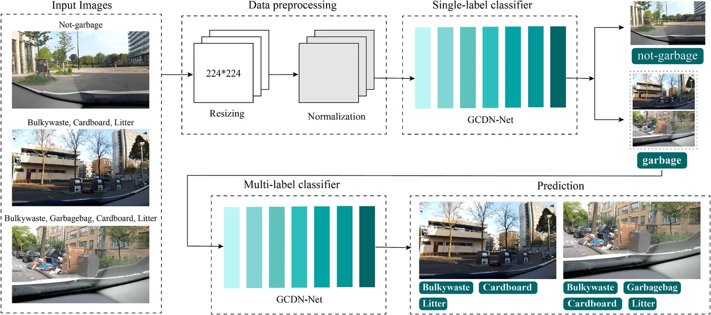
Growing cities produce more waste, and about a third of global waste is disposed of without proper sorting. Automated sorting and street cleaning need models that recognise waste in real scenes, where several types often lie together against busy backgrounds. This study proposed GCDN-Net, which combines DenseNet201 and Inception-v3. A first stage separates street images with and without garbage, and a second stage names the garbage types present.
- Clean and prepare street images
- Detect garbage in each image
- Name the waste types present
Cleaning and preparing the street images
Waste Management · 2024
The study used the public GIGO dataset of 25,000 images taken by two car-mounted cameras on city streets: 9,352 with garbage and 15,648 without. Garbage images carry labels for four types, and one image can show several: bulky waste such as sofas and fridges, garbage bags, cardboard and litter.
Faces and number plates in the dataset are hidden by grey or yellow boxes, which a model could mistake for garbage. About 3,000 affected images were removed, leaving 7,410 garbage images, and 8,760 images without garbage were sampled to balance the classes. Each dataset was split 70%, 10% and 20% for training, validation and testing, and every model was evaluated with five-fold cross-validation.
Horizontal flips and rotations of up to 30 degrees raised the training images to about 5,000 per class. Images were resized to 224 × 224 pixels and normalised with the dataset’s mean and standard deviation.
- Cleaned images used
- 16,170
- Garbage types labelled
- 4
- Cross-validation
- 5-fold
| Training | Validation | Test | |
|---|---|---|---|
| Garbage | 5,187 | 741 | 1,482 |
| Not garbage | 6,132 | 846 | 1,752 |
| Garbage bag | 1,307 | 182 | 392 |
| Cardboard | 2,853 | 414 | 832 |
| Bulky waste | 3,249 | 466 | 933 |
| Litter | 2,447 | 343 | 686 |
Fusing two pretrained networks to detect garbage
Single-label classification
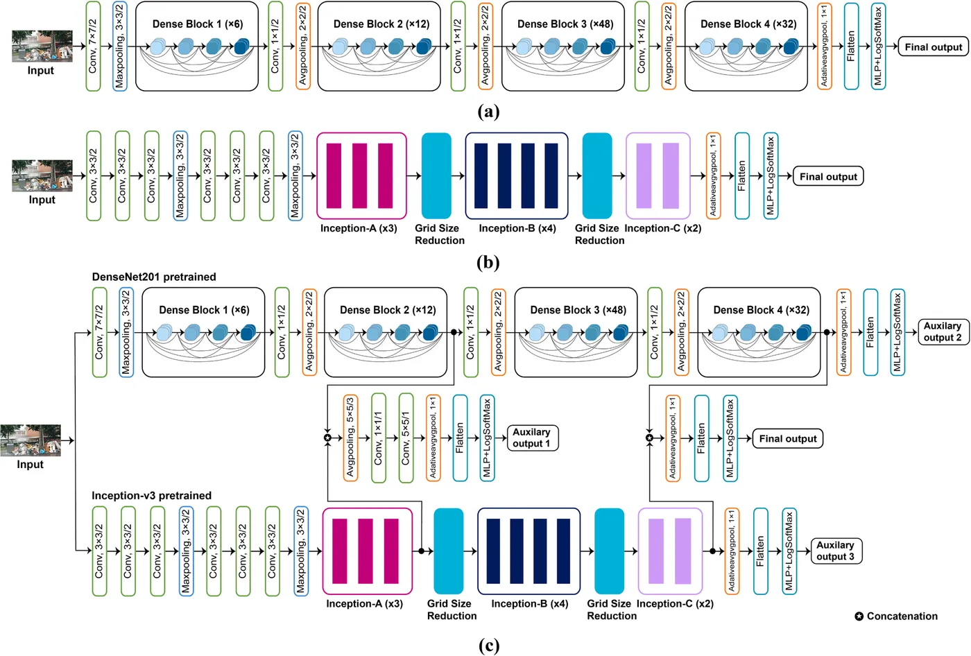
Four ImageNet-pretrained networks were compared first: ResNet50, MobileNetV2, DenseNet201 and Inception-v3. DenseNet201 and Inception-v3 performed best, so GCDN-Net combines them. The features from the last layers of both networks are joined before the final classifier.
Three auxiliary outputs add deep supervision. One joins features from the middle of both networks, and the others come from the end of each network. The auxiliary losses get smaller weights the shallower they are, and the model was trained with the Adam optimiser at a learning rate of 0.0001.
GCDN-Net separated garbage from non-garbage images with 95.77% accuracy and 95.54% specificity. Joining the two networks raised accuracy from 91.60% for Inception-v3 alone to 93.15%, one auxiliary output raised it to 94.72%, and three auxiliary outputs gave the final result.
- Accuracy
- 95.77%
- Specificity
- 95.54%
- Accuracy gain over Inception-v3 alone
- 4.17 points
| Accuracy | Precision | Specificity | F1 score | |
|---|---|---|---|---|
| MobileNetV2 | 87.61 | 87.63 | 87.56 | 87.62 |
| ResNet50 | 90.38 | 90.39 | 90.05 | 90.37 |
| DenseNet201 | 90.69 | 90.69 | 90.34 | 90.67 |
| Inception-v3 | 91.60 | 91.60 | 91.42 | 91.60 |
| GCDN-Net, no auxiliary output | 93.15 | 93.17 | 93.85 | 93.14 |
| GCDN-Net, one auxiliary output | 94.72 | 94.73 | 94.53 | 94.73 |
| GCDN-Net, three auxiliary outputs | 95.77 | 95.78 | 95.54 | 95.77 |
Naming the types of waste in each image
Multi-label classification
The 7,410 garbage images then went to a multi-label GCDN-Net. A sigmoid output with binary cross-entropy loss treats each of the four types as a separate yes-or-no decision, so one image can receive several labels.
Across the four types, GCDN-Net reached a mean average precision of 0.69 and an F1 score of 75.01%. Bulky waste was recognised best, with a mean average precision of 0.73 and an F1 score of 80.23%. Garbage bags were hardest: they made up only 13.33% of the labels and are often small in the frame. An earlier study on the same dataset reported a mean average precision of 0.47 with a vision transformer.
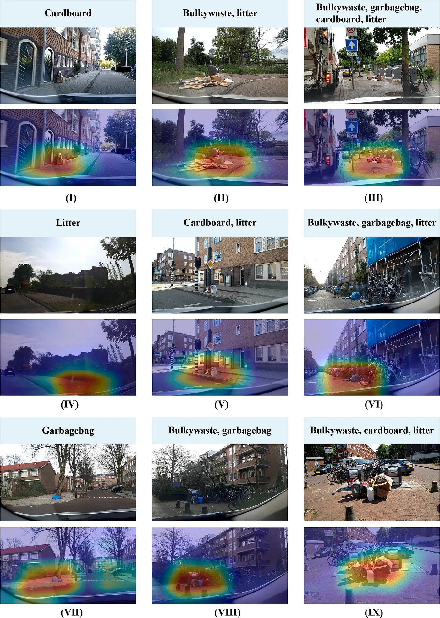
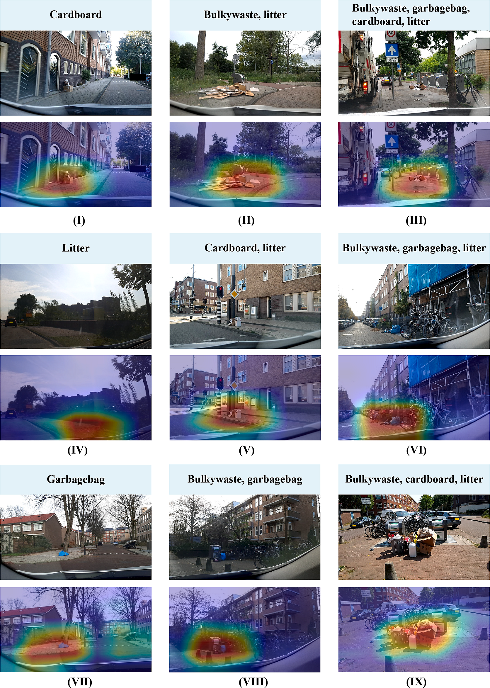
Score-CAM heatmaps showed which parts of each image drove the predictions. For images with one, two or more waste types, the heatmaps concentrated on the garbage rather than on surrounding buildings, vehicles or trees.
- Mean average precision
- 0.69
- F1 score
- 75.01%
- F1 score for bulky waste
- 80.23%
| Mean average precision | Precision | Recall | F1 score | |
|---|---|---|---|---|
| Bulky waste | 0.73 | 73.97 | 87.69 | 80.23 |
| Cardboard | 0.73 | 73.96 | 81.91 | 77.69 |
| Litter | 0.66 | 69.74 | 72.50 | 70.96 |
| Garbage bag | 0.56 | 71.05 | 57.05 | 63.12 |
| Overall | 0.69 | 72.56 | 78.32 | 75.01 |
My contribution
I helped develop the framework and contributed to the evaluation, experimental analysis, interpretation and manuscript review.
Study scope
All images came from one dataset of urban street scenes, and about 3,000 were removed because privacy boxes could be mistaken for garbage. Without bounding boxes, the model reports which waste types are present but cannot locate or count individual items, and busy backgrounds made multi-label classification harder.
Publications
- GCDN-Net: Garbage classifier deep neural network for recyclable urban waste managementWaste Management · 2024